Tutorial: Data Streams
This tutorial shows how you can process real-world data streams of position data with BBoxDB Streams. BBoxDB Streams is a distributed stream processing system that allows the handling of multi-dimensional data. The system is an extension of BBoxDB. BBoxDB is a key-bounding-box value store, which allows the efficient storage and retrieval of multi-dimensional data.
The efficient spatial join between a data stream and n-dimensional big data is a unique feature of BBoxDB Streams. Data of multiple-tables of the same dimensionality can be stored co-partitioned. This means that the data of the two tables are partitioned and distributed in the same way. Spatial joins can be efficiently executed, no data needs to be transferred between the nodes to calculate the join.
Process a Real-World Stream of Public Transport Data
The position data of public transport vehicles in Sydney are used as the real-world data stream. Continuous queries such as range queries or spatial joins between the stream elements and n-dimensional data will be performed. The data stream can be fetched from the open data website of the public transport company in New South Wales. Spatial data from the OpenStreetMap project is used for the static dataset. Queries such as:
- Which bus / train / ferry is currently located in a given query rectangle (continuous range query)?
- Which bus is currently located on a Bridge (continuous spatial join query)?
- Which bus is currently driving through a forest (continuous spatial join query)?
- Which bus is currently located on a particular road (continuous spatial join query)?

The buses in Sydney, interactively shown as a continuous range query in the GUI of BBoxDB.
Note: For more information, have a look at our Stream Processing paper, presented at EDBT 2021.
Download and Convert Open Street Map Data into GeoJSON
For performing the continuous spatial joins, you need to import the spatial dataset of the area first. Please download the complete Planet dataset or the Australia dataset in .osm.pbf format.
After the dataset is downloaded, it needs to be converted into GeoJSON elements. This can be done by calling the following command:
$BBOXDB_HOME/bin/osm_data_converter.sh -input <your-dataset>.osm.pbf -backend bdb -workfolder /tmp/work -output <outputdir>
After the command finishes, several files in the output folder like ROADS or FORSTS are generated. These files contain the spatial data of the corresponding OpenStreetMap elements as GeoJSON elements. Each like of the file contains one GeoJSON element. For example, one entry might look like (the entry is formatted and split-up into multiple lines for improved reading):
{
   "geometry":{
      "coordinates":[
         [
            151.2054938,
            -33.9045641
         ],
         [
            151.2056594,
            -33.9047744
         ],
         [
            151.20597560000002,
            -33.905176000000004
         ],
         [
            151.2063965,
            -33.9057107
         ],
         [
            151.20641930000002,
            -33.905739700000005
         ]
      ],
      "type":"LineString"
   },
   "id":756564602,
   "type":"Feature",
   "properties":{
      "surface":"paved",
      "hgv":"destination",
      "maxspeed":"40",
      "name":"Elizabeth Street",
      "highway":"residential",
      "maxweight":"3"
   }
}
See this page for more information about the data converter.
Pre-partition the Space and Import the GeoJSON Data
After the spatial data is converted into GeoJSO, you can import the data by calling the following command:
$BBOXDB_HOME/bin/import_osm.sh <outputdir> nowait
The command performs the following tasks:
- The distribution group
osm(short for OpenStreetMap) is created. - The tables
osm_roadandosm_forstare created. - A sample is taken from the data, and the space is pre-partitioned into 10 distribution regions.
- The spatial data is read and imported into BBoxDB.
Hint: When you remote the nowait parameter from the command, the command will stop after each step, and you can analyze the output.
Create an Account to Access the Data Stream
To fetch the data stream of the vehicles in Sydney, you have to apply for a API key. This can be done at the following website. Please create an API key that is capable of accessing the “GTFS real-time” encoded data stream of the vehicles.
Import the Datastream
To import the data stream, the following tables need to be created in BBoxDB. In these tables, the data stream elements will be stored. All tables are part of the distribution group osm.
$BBOXDB_HOME/bin/cli.sh -action create_table -table osmgroup_lightrail
$BBOXDB_HOME/bin/cli.sh -action create_table -table osmgroup_buses
$BBOXDB_HOME/bin/cli.sh -action create_table -table osmgroup_metro
$BBOXDB_HOME/bin/cli.sh -action create_table -table osmgroup_nswtrains
$BBOXDB_HOME/bin/cli.sh -action create_table -table osmgroup_ferries
$BBOXDB_HOME/bin/cli.sh -action create_table -table osmgroup_trains
Afterward, you can start the import of the data stream into BBoxDB.
$BBOXDB_HOME/bin/bboxdb_execute.sh org.bboxdb.tools.network.CaptureAUTransportStream "<Your-API-Key>" lightrail:buses:metro:nswtrains:ferries:trains <cluster-contact-point> <your-cluster-name> osmgroup 2
Note: The 2 at the end of the command means that the data source is pulled every 2 seconds, and the data is imported into BBoxDB.
Perform Queries on the Data Stream
On the CLI, you can perform the following continuous query to see all data of the data stream. The provided bounding box for the range query [[-35,-30]:[150,152]] covers the area of Australia.
$BBOXDB_HOME/bin/cli.sh -action query_continuous -table osmgroup_buses -bbox [[-35,-30]:[150,152]]
For more queries, please use the GUI of BBoxDB. You can start the GUI by executing:
$BBOXDB_HOME/bin/gui.sh
Open the query view on the GUI and navigate to Sydney. In the GUI the queries from the introduction are pre-defined. In addition, you can execute individual queries.
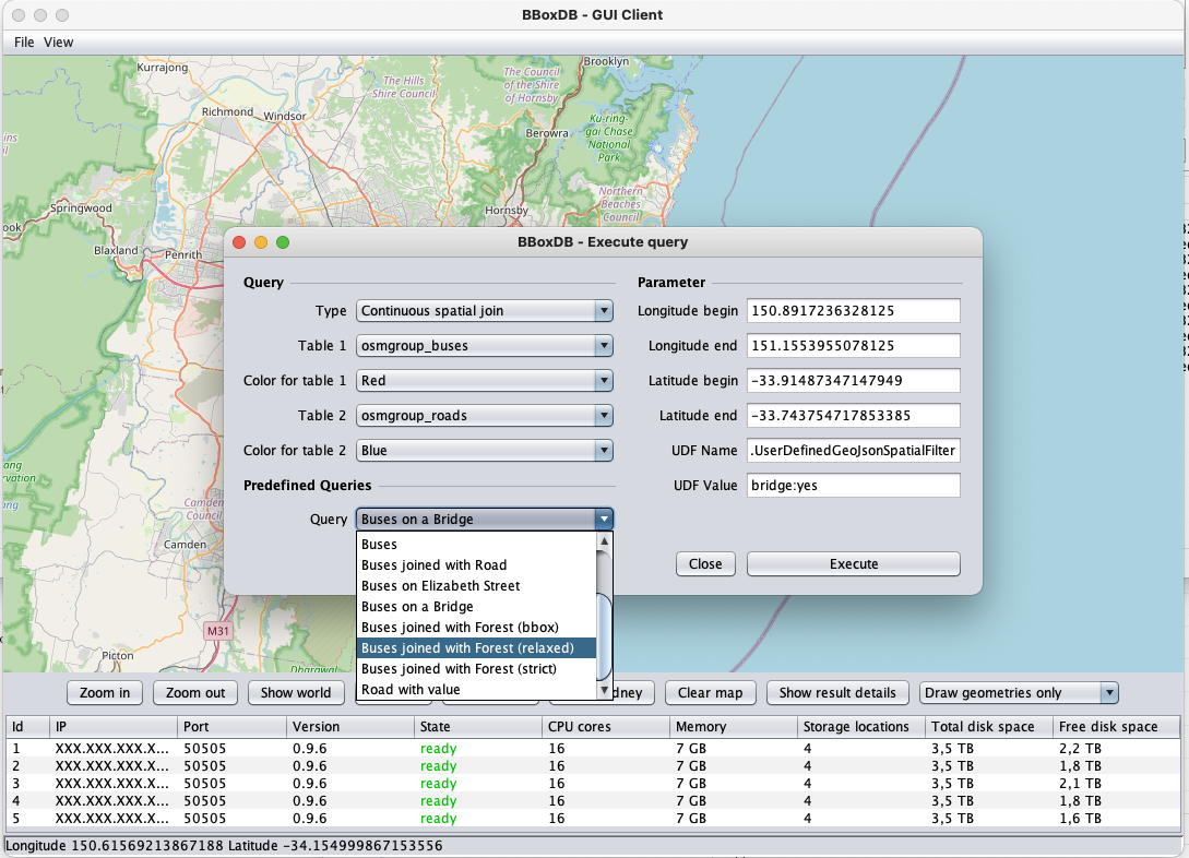
The predefined queries in the GUI.
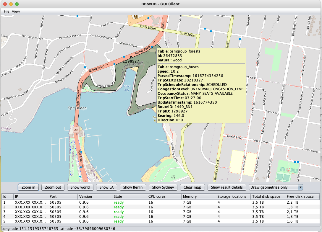
A bus in a forest.
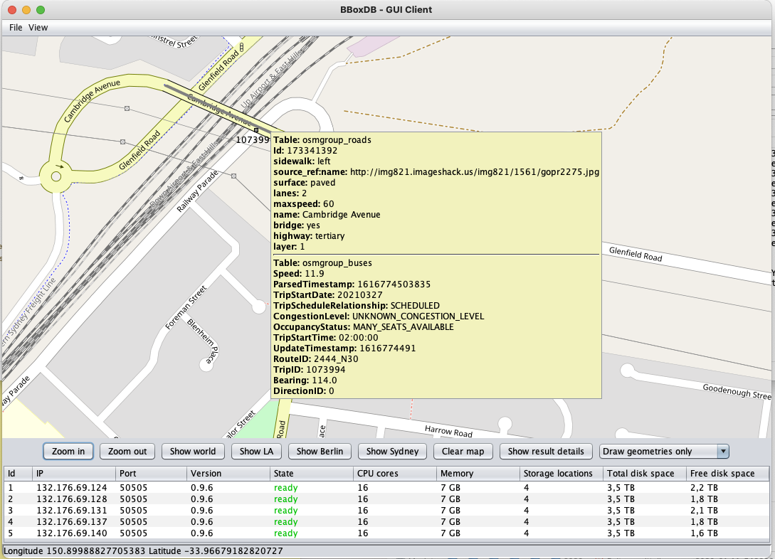
A bus on a bridge.
Process a Real-World Stream of ADS-B Data
In this part of the tutorial, a stream of ADS-B data (Automatic Dependent Surveillance-Broadcast) is processed with BBoxDB Streams. ADS-B data contains data of aircraft (containing the position, height, heading, call sign, and much more). The GUI of BBoxDB is used to show live data of aircraft. Continuous queries such as which aircraft is currently in the airspace over Berlin? can be performed.
In this tutorial, the data is fetched from two input sources:
- A local ADS-B receiver
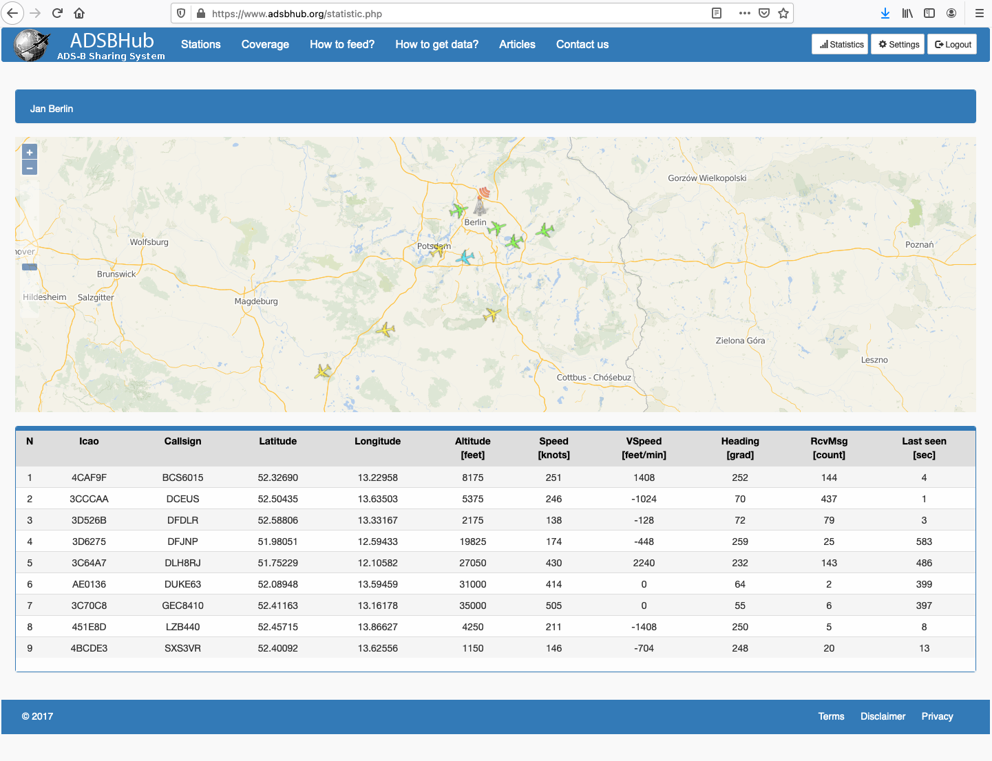
- The website ADSBHub.org
As the local ADS-B receiver, an AirNav USB-Stick is used in this tutorial. This is a small USB-receiver that is delivered together with an antenna. The receiver can be bought at websites such as Amazon or eBay.

A receiver that is capable of capturing ADS-B messages.
The local ADS-B receiver captures the data of aircraft in the region of the antenna. Unfortunately, the antenna can only capture transmissions in a radius of a few miles. To get an ADS-B data stream covering a larger region, websites such as adsbhub.org can be used. By uploading your received data, you can fetch the data from all registered stations.
To access this data stream of adsbhub.org, you have to upload your received ADS-B data stream to adsbhub.org website. Afterward, you have access to the data of all other stations that are transmitting data to adsbhub.org.
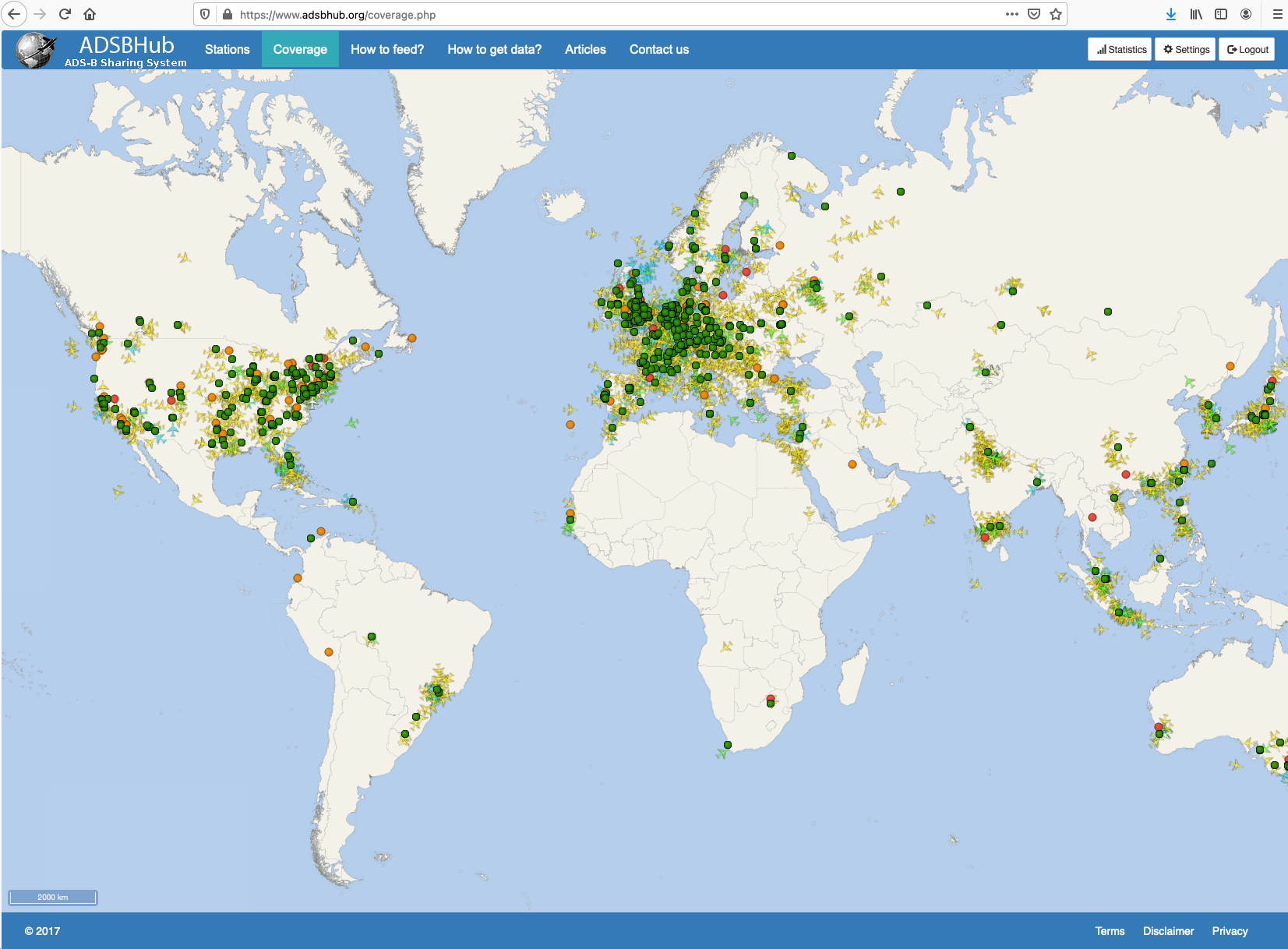
The coverage of the adsbhub.org website.
Install the Needed Software to Handle the ADS-B data
After the ADS-B receiver is connected to your PC, you need to download and compile the program dump1090. The program is capable of decoding ADS-B data.
git clone https://github.com/flightaware/dump1090.git
cd dump1090
apt-get install librtlsdr-dev
make
Execute dump1090
Some Linux distributions load some kernel drivers automatically to support the USB stick. These drivers prevent that dump1090 can access the receiver directly. Please unload the driver first to ensure that dump1090 works correctly.
rmmod rtl2832 rtl2832_sdr rtl2832 dvb_core dvb_usb_v2 dvb_usb_rtl28xxu
Afterward, dump1090 can be started, by executing:
./dump1090 --interactive --device-type rtlsdr --net
The output for the program should look as follows. In the example, eight aircraft are shown.
 Tot:   8 Vis:   8 RSSI: Max -26.0+ Mean -31.5 Min -34.7-  MaxD:    0.0nm+     /
 Hex    Mode  Sqwk  Flight   Alt    Spd  Hdg    Lat      Long   RSSI  Msgs  Ti
────────────────────────────────────────────────────────────────────────────────
 3CCCAA A0    5004           12750  373  072                   -32.6    44 10
 4BA8C5 A2    1000  THY2SY    4275  208  248   52.458   13.866 -31.2   156 51
 3944F3 A0    1000  AFR91RW  38975  473  073                   -32.8    27 23
 3D6275 A2          DFJNP     9800  151  259   52.037   13.088 -32.0    88 04
 4BCDE3 A0                                                     -34.7-    4 42
 5140A8 A0    3213           34325  382  256   52.148   15.322 -32.4   332 11
 3C64A7 A2    1000  DLH8RJ   13175  349  233   52.185   13.021 -26.0+ 2350 08
 3D2C04 S     7372  DEOXO     1200                             -30.7  1352 58
Upload the Captured Data to adsbhub.org
The program dump1090 was started in network mode by specifying the --net parameter. This means that the program opens several ports and provides the data stream in various formats on these ports. By calling the following command, the data stream is read from the port 30003.
nc localhost 30003
The command should show an output that looks like the following example. This is the ADS-B data encoded in SBS-format. More about this data format can be found at the following website.
MSG,5,1,1,3D2C04,1,2021/03/31,10:59:34.052,2021/03/31,10:59:34.087,,1600,,,,,,,0,,0,
MSG,8,1,1,471F8C,1,2021/03/31,10:59:34.141,2021/03/31,10:59:34.195,,,,,,,,,,,,0
MSG,8,1,1,471F8C,1,2021/03/31,10:59:34.177,2021/03/31,10:59:34.200,,,,,,,,,,,,0
MSG,8,1,1,471F8C,1,2021/03/31,10:59:34.186,2021/03/31,10:59:34.201,,,,,,,,,,,,0
MSG,8,1,1,471F8C,1,2021/03/31,10:59:34.187,2021/03/31,10:59:34.201,,,,,,,,,,,,0
MSG,5,1,1,3D2C04,1,2021/03/31,10:59:34.309,2021/03/31,10:59:34.359,,1600,,,,,,,0,,0,
MSG,7,1,1,5140A8,1,2021/03/31,10:59:34.523,2021/03/31,10:59:34.577,,37500,,,,,,,,,,
MSG,4,1,1,3C64A7,1,2021/03/31,10:59:34.637,2021/03/31,10:59:34.687,,,244,235,,,2368,,,,,0
MSG,5,1,1,3D2C04,1,2021/03/31,10:59:35.001,2021/03/31,10:59:35.020,,1600,,,,,,,0,,0,
MSG,5,1,1,3D2C04,1,2021/03/31,10:59:35.052,2021/03/31,10:59:35.073,,1600,,,,,,,0,,0,
MSG,7,1,1,3C64A7,1,2021/03/31,10:59:35.353,2021/03/31,10:59:35.398,,6725,,,,,,,,,,
MSG,8,1,1,3C64A7,1,2021/03/31,10:59:35.456,2021/03/31,10:59:35.506,,,,,,,,,,,,0
MSG,8,1,1,3C64A7,1,2021/03/31,10:59:35.474,2021/03/31,10:59:35.509,,,,,,,,,,,,0
MSG,8,1,1,3C64A7,1,2021/03/31,10:59:35.502,2021/03/31,10:59:35.512,,,,,,,,,,,,0
MSG,6,1,1,471F8C,1,2021/03/31,10:59:35.559,2021/03/31,10:59:35.566,,,,,,,,0514,0,0,0,
MSG,3,1,1,3C64A7,1,2021/03/31,10:59:35.671,2021/03/31,10:59:35.724,,6725,,,52.30884,13.29165,,,0,,0,0
MSG,4,1,1,3C64A7,1,2021/03/31,10:59:35.676,2021/03/31,10:59:35.725,,,246,235,,,2368,,,,,0
MSG,8,1,1,3C64A7,1,2021/03/31,10:59:35.867,2021/03/31,10:59:35.889,,,,,,,,,,,,0
MSG,5,1,1,3C64A7,1,2021/03/31,10:59:35.870,2021/03/31,10:59:35.889,,6750,,,,,2208,,0,,0,
MSG,5,1,1,3C64A7,1,2021/03/31,10:59:35.888,2021/03/31,10:59:35.942,,6750,,,,,,,0,,0,
When the local data stream can be accessed successfully, you should register your receiver at adsbhub.org. Afterward, the data stream can be uploaded to the website. This can be done by the script upload_to_adsbhub.sh, which is contained in the BBoxDB repository. The script automatically re-starts the upload when your Internet connection becomes unavailable.
wget https://raw.githubusercontent.com/jnidzwetzki/bboxdb/master/misc/upload_to_adsbhub.sh
chmod +x ./upload_to_adsbhub.sh
./upload_to_adsbhub.sh
When everything works correctly, you should see your received data under the following URL.
Your station data at the website adsbhub.org.
Now you can access the complete ADS-B data stream of the adsbhub.org website. You can verify this by executing:
nc data.adsbhub.org 5002
The command should show you the current ADS-B data stream of adsbhub.org. The data stream looks like this and contains the data of airplanes of the whole world.
MSG,3,0,0,E495D8,0,2021/03/31,09:35:22.000,2021/03/31,09:35:22.000,,38000,,,-22.659973,-44.255676,,,,,,
MSG,4,0,0,E495D8,0,2021/03/31,09:35:22.000,2021/03/31,09:35:22.000,,,400.870300,249.711609,,,0,,,,,
MSG,1,0,0,E495DF,0,2021/03/31,09:35:22.000,2021/03/31,09:35:21.000,AZU4399,,,,,,,,,,,
MSG,3,0,0,E495DF,0,2021/03/31,09:35:22.000,2021/03/31,09:35:21.000,,15650,,,-22.554810,-46.767151,,,,,,
MSG,4,0,0,E495DF,0,2021/03/31,09:35:22.000,2021/03/31,09:35:21.000,,,313.209198,216.430862,,,-1216,,,,,
MSG,1,0,0,E495F9,0,2021/03/31,09:35:22.000,2021/03/31,09:35:21.000,GLO1547,,,,,,,,,,,
MSG,3,0,0,E495F9,0,2021/03/31,09:35:22.000,2021/03/31,09:35:21.000,,11950,,,-23.055298,-46.552124,,,,,,
MSG,4,0,0,E495F9,0,2021/03/31,09:35:22.000,2021/03/31,09:35:21.000,,,293.163788,199.114807,,,-1472,,,,,
MSG,1,0,0,E4966D,0,2021/03/31,09:35:22.000,2021/03/31,09:35:21.000,AZU4514,,,,,,,,,,,
MSG,3,0,0,E4966D,0,2021/03/31,09:35:22.000,2021/03/31,09:35:21.000,,41000,,,-25.244934,-47.058411,,,,,,
MSG,4,0,0,E4966D,0,2021/03/31,09:35:22.000,2021/03/31,09:35:21.000,,,483.359070,35.399883,,,64,,,,,
Prepare BBoxDB and Import the Data Stream
After the data stream can be fetched, it’s time to prepare BBoxDB to handle the data stream. In the first step, the needed distribution group (osmgroup in this example) is created together with the table for the adsb data osmgroup_adsb.
$BBOXDB_HOME/bin/cli.sh -action create_dgroup -dgroup osmgroup -dimensions 2 -maxregionsize 1024
$BBOXDB_HOME/bin/cli.sh -action create_table -table osmgroup_adsb
After BBoxDB is prepared, the import of the ADS-B data stream can be performed by executing the following command. The command fetches the data stream and converts the ADS-B data in the SBS format into GeoJSON elements, which can be processed later by the GUI of BBoxDB.
$BBOXDB_HOME/bin/bboxdb_execute.sh org.bboxdb.tools.network.CaptureADSB <cluster-contact-point> <your-cluster-name> osmgroup_adsb
Perform Queries on The GUI
So, the data stream is available in BBoxDB; queries on the data can now be performed. This can be done by the GUI of BBoxDB. You can start the GUI by executing:
$BBOXDB_HOME/bin/gui.sh
Open the query view on the GUI and perform range queries or continuous range queries on the osmgroup_adsb table.
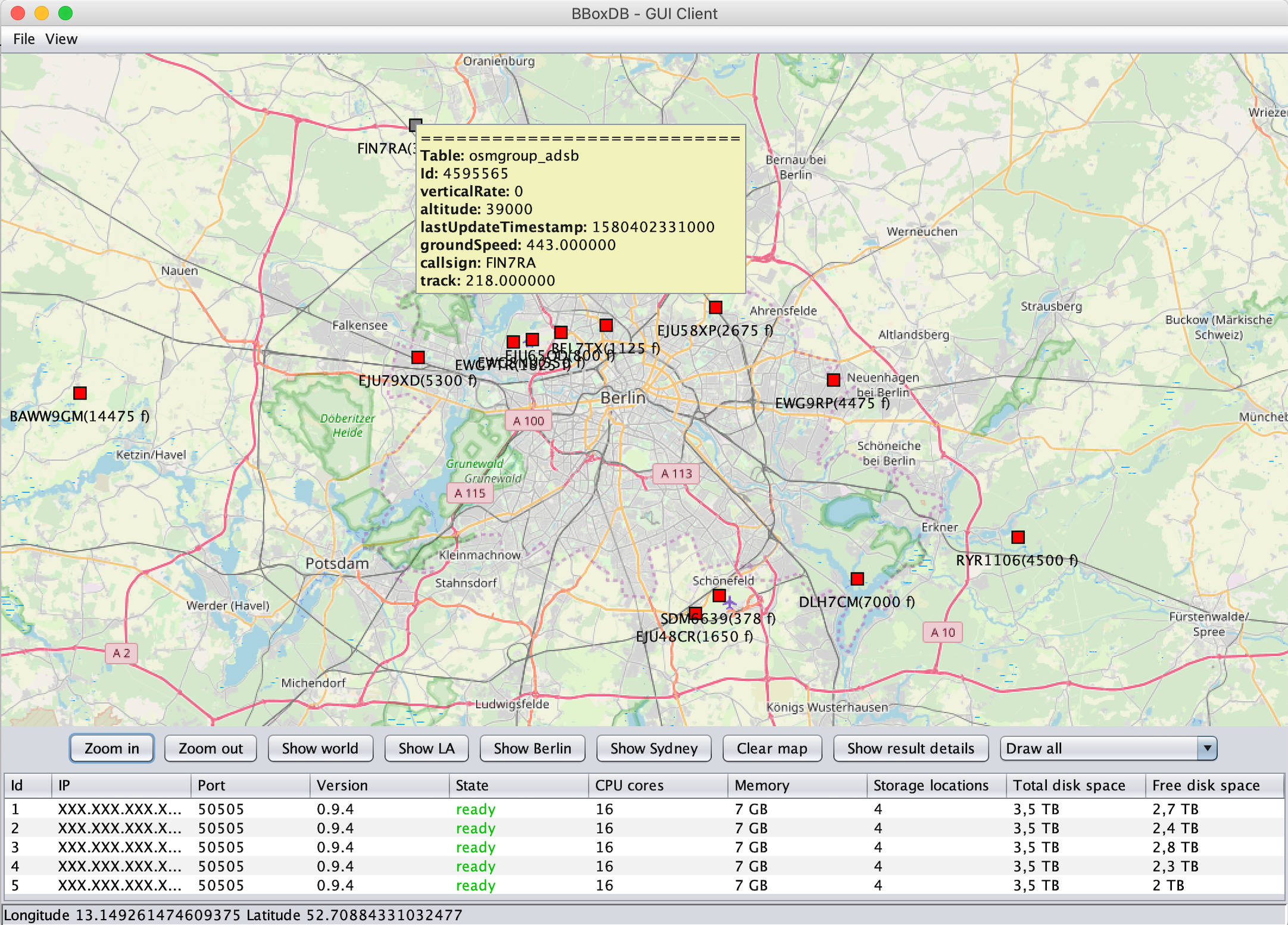
A continuous range query on the ADS-B data stream in the area of Berlin, shown in the GUI of BBoxDB.
Each rectangle in the screenshot is one aircraft. Below each aircraft, the call sign and the altitude are shown. Placing the mouse over the aircraft will open a tooltip containing additional information like the heading or the speed.
Work with BerlinMod Simulation Data
Data generated by the BerlinMod benchmark can be used to simulate a fleet of moving vehicles in Berlin, Germany. The BerlinModPlayer takes the generated static data and generates a real-time data stream of position data.
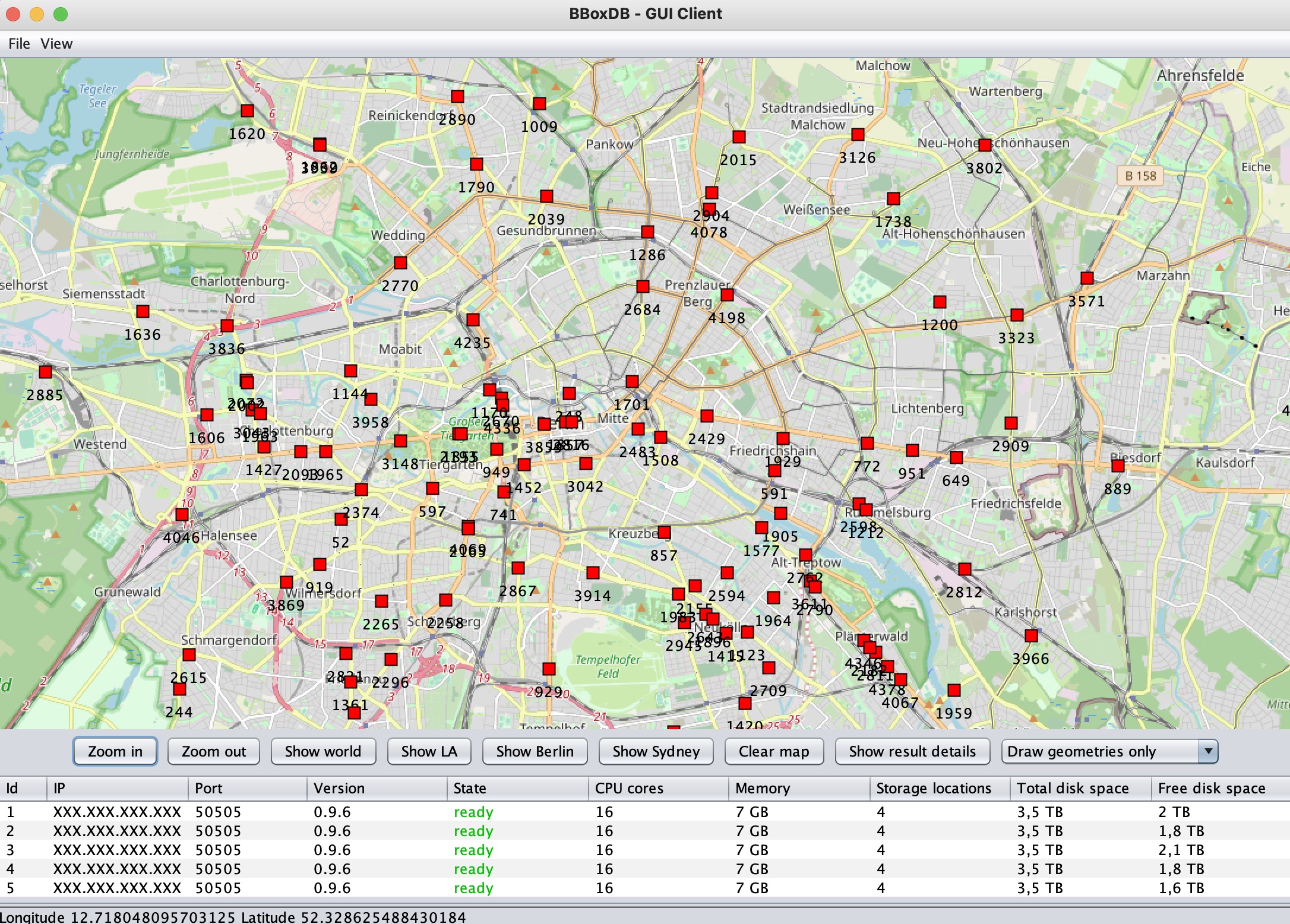
A continuous range query on the BerlinMod data stream in the area of Berlin, shown in the GUI of BBoxDB.
Generate Simulation Data
A working installation of SECONDO is needed to generate the needed simulation data. After SECONDO is installed, perform the following steps to install and configure the BerlinMod Benchmark.
cd $SECONDO_BUILD_DIR/bin
wget https://github.com/secondo-database/secondo-database.github.io/raw/main/BerlinMOD/Scripts_OptimizerCompilant-2019-08-28.zip
unzip Scripts_OptimizerCompilant-2019-08-28.zip

# Adjust in scripts/BerlinMOD_DataGenerator.SEC
let P_NUMCARS = 1000;
let P_NUMDAYS = 10;
Afterward, the simulation data can be calculated by performing the following command:
./SecondoTTYNT -i scripts/BerlinMOD_DataGenerator.SEC
Now, the generated data can be exported to disk. This is performed by executing the following commands. In contrast to the regular export which BerlinMod performs, the coordinates are converted into the WGS84 coordinate system.
./SecondoTTYNT

open database berlinmod;

query dataMtrip feed
  project[Moid,Tripid, Trip]
  projectextendstream[Moid, Tripid; Unit : units(.Trip)]
  projectextend [ Moid, Tripid; Tstart : inst(initial(.Unit)),
  Tend : inst(final(.Unit)),
  Xstart : getx(berlin2wgs(val(initial(.Unit)))),
  Ystart : gety(berlin2wgs(val(initial(.Unit)))),
  Xend : getx(berlin2wgs(val(final(.Unit)))),
  Yend : gety(berlin2wgs(val(final(.Unit)))) ]
  sortby[Tstart]
csvexport['trips.csv',FALSE,TRUE] count;
Download and Install the BerlinModPlayer
To download and compile the BerlinModPlayer, please execute the following commands:
git clone https://github.com/jnidzwetzki/berlinmodplayer.git
cd berlinmodplayer/src
make
Prepare BBoxDB for the Stream
Now, BBoxDB can be prepared for the import of the data stream. A proper distribution group and a table for the data stream have to be created:
$BBOXDB_HOME/bin/cli.sh -action create_dgroup -dgroup osmgroup -dimensions 2 -maxregionsize 10485760
$BBOXDB_HOME/bin/cli.sh -action create_table -table osmgroup_berlinmod
Perform the Simulation
To perform the simulation, the data importer of BBoxDB has to be started. The following command opens the port 10000/tcp, parses the data that is written to the port, and writes the data to the BBoxDB table osmgroup_berlinmod.
$BBOXDB_HOME/bin/bboxdb_execute.sh org.bboxdb.tools.network.SocketImporter 10000 132.176.69.124:50181 mycluster osmgroup_berlinmod berlinmod_player dynamic true
Afterward, the simulation can be started by executing:
./bmodplayer -i <path_to_berlin_mod>/trips_wgs.csv -u tcp://localhost/10000 -s adaptive -r 1 -f 2 -b '2007-05-28 06:10:14'
For more details about the used parameter, have a look at the documentation of the BerlinModPlayer.
Now you can start the GUI of BBoxDB as described in the last two sections. The data stream is written to the table osmgroup_berlinmod; continuous queries can be performed on this table.